R with RStudio: getting started - R workshops at ResBaz Qld 2021

R + RStudio

The R programming language is a language used for calculations, statistics, visualisations and many more data science tasks.

RStudio is an open source Integrated Development Environment (IDE) for R, which means it provides many features on top of R to make it easier to write and run code.

R’s main strong points are:

Open Source: you can install it anywhere and adapt it to your needs;
Reproducibility: makes an analysis repeatable by detailing the process in a script;
Customisable: being a programming language, you can create your own custom tools;
Big data: it can handle very large datasets;
Many formats: it can read and write most file formats;
Large ecosystem: packages allow you to extend R for thousands of different analyses.

The learning curve will be steeper than point-and-click tools, but as far as programming languages go, R is more user-friendly than others.

Installation

For this course, you need to have both R and RStudio installed (installation instructions).

Open RStudio

If you are using your own laptop please open RStudio
- Make sure you have a working Internet connection

What are we going to learn?

This session is designed to get straight into using R in a short amount of time, which is why we won’t spend too much time on the smaller details that make the language.

During this session, you will:

Create a project for data analysis
Create a folder structure
Know where to find help
Learn about a few useful functions
Generate a data visualisation
Create a script
Import a dataset
Understand the different RStudio panels
Use a few shortcuts
Know how to extend R with packages

R Projects

Let’s first create a new project:

Click the “File” menu button (top left corner), then “New Project”
Click “New Directory”
Click “New Project”
In “Directory name”, type the name of your project, for example “YYYY-MM-DD_rstudio-intro”
Browse and select a folder where to locate your project (~ is your home directory). For example, a folder called “r-projects”.
Click the “Create Project” button

R Projects make your work with R more straight forward, as they allow you to segregate your different projects in separate folders. You can create a .Rproj file in a new directory or an existing directory that already has R code and data. Everything then happens by default in this directory. The .Rproj file stores information about your project options, and allows you to go straight back to your work.

Maths and objects

The console (usually at the bottom right in RStudio) is where most of the action happens. In the console, we can use R interactively. We write a command and then execute it by pressing Enter.

In its most basic use, R can be a calculator. Try executing the following commands:

10 - 2

## [1] 8

3 * 4

## [1] 12

2 + 10 / 5

## [1] 4

Those symbols are called “binary operators”: we can use them to multiply, divide, add, subtract and exponentiate. Once we execute the command (the “input”), we can see the result in the console (the “output”).

What if we want to keep reusing the same value? We can store data by creating objects, and assigning values to them with the assignment operator <-:

num1 <- 42
num2 <- num1 / 9
num2

## [1] 4.666667

We can also store text data:

sentence <- "Hello World!"
sentence

## [1] "Hello World!"

You should now see your objects listed in you environment pane (top right).

As you can see, you can store different kinds of data as objects. If you want to store text data (a “string of characters”), you have to surround it by quotes.

Depending on the kind of data, some operations will be possible, and others will yield an error:

> sentence * 2
Error in sentence * 2 : non-numeric argument to binary operator

In the error message above, R is telling us that using the multiplication operator * can only deal with numeric data. sentence is of “character” type.

You can use the shortcut Alt+- to type the assignement operator quicker.

Functions

An R function is a little program that does a particular job. It usually looks like this:

<functionname>(<argument(s)>)

Arguments tell the function what to do. Some functions don’t need arguments, others need one or several, but they always need the parentheses after their name.

For example, try running the following command:

round(num2)

## [1] 5

The round() function rounds a number to the closest integer. The only argument we give it is num2, the number we want to round.

If you scroll back to the top of your console, you will now be able to spot functions in the text.

Help

What if we want to learn more about a function?

There are two main ways to find help about a specific function in RStudio:

the shortcut command: ?functionname
the keyboard shortcut: press F1 with your cursor in a function name

Let’s look through the documentation for the round() function:

?round

As you can see, different functions might share the same documentation page.

There is quite a lot of information in a function’s documentation, but the most important bits are:

Description: general description of the function(s)
Usage: overview of what syntax can be used
Arguments: description of what each argument is
Examples: some examples that demonstrate what is possible

See how the round() function has a second argument available? Try this now:

round(num2, digits = 2)

## [1] 4.67

We can change the default behaviour of the function by telling it how many digits we want after the decimal point, using the argument digits. And if we use the arguments in order, we don’t need to name them:

round(num2, 2)

## [1] 4.67

Challenge 1 – Finding help

Use the help pages to find out what these functions do, and try executing commands with them:

c()
rep.int()
mean()
rm()

c() combines the arguments into a vector. In other words, it takes any number of arguments (hence the ...), and stores all those values together, as one single object. For example, let’s store the ages of our pet dogs in a new object:

ages <- c(4, 10, 2, NA, 3)

You can store missing data as NA.

We can now reuse this vector, and calculate their human age¹:

ages * 7

## [1] 28 70 14 NA 21

Or use it in a logical operation:

ages > 3

## [1]  TRUE  TRUE FALSE    NA FALSE

R can create visualisations with functions too. Try a bar plot of your dogs’ ages with the barplot() function:

barplot(ages)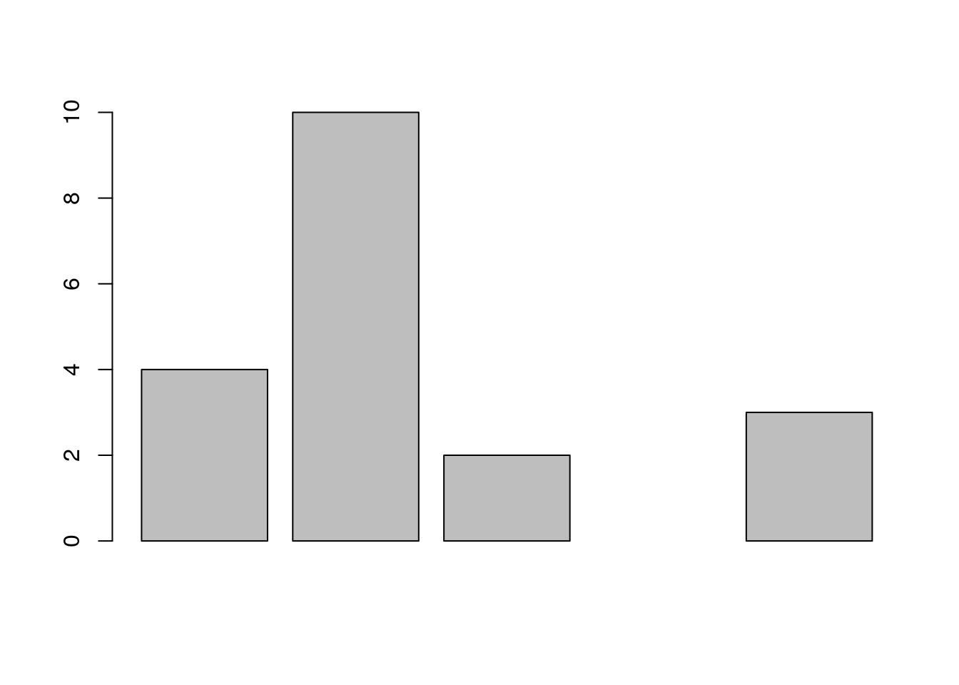

Remember that vectors need to stick to one kind of data, so the following command:

things <- c(1, TRUE, "Hi!")

… will coerce all elements to one single type: the “character” type.

Other data structures are available for storing your data in R: lists (very flexible) and data frames (like spreadsheets), as well as matrices (with one data type, like vectors). We will talk about data frames in our example project.

Moving on to our second function: rep.int() also creates vectors, but it is designed to easily replicate values. For example, if you find something very funny:

rep.int("Ha!", 30)

##  [1] "Ha!" "Ha!" "Ha!" "Ha!" "Ha!" "Ha!" "Ha!" "Ha!" "Ha!" "Ha!" "Ha!" "Ha!"
## [13] "Ha!" "Ha!" "Ha!" "Ha!" "Ha!" "Ha!" "Ha!" "Ha!" "Ha!" "Ha!" "Ha!" "Ha!"
## [25] "Ha!" "Ha!" "Ha!" "Ha!" "Ha!" "Ha!"

The next function, mean(), returns the mean of a vector of numbers:

mean(ages)

## [1] NA

What happened there?

We have an NA value in the vector, which means the function can’t tell what the mean is. If we want to change this default behaviour, we can use an extra argument: na.rm, which stands for “remove NAs”.

mean(ages, na.rm = TRUE)

## [1] 4.75

In our last command, if we hadn’t named the na.rm argument, R would have understood TRUE to be the value for the trim argument!

Finally, rm() removes an object from your environment (remove() and rm() point to the same function). For example:

rm(num1)

R does not check if you are sure you want to remove something! As a programming language, it does what you ask it to do, which means you might have to be more careful. But you’ll see later on that, when working with scripts, this is less of a problem.

Let’s do some more complex operations by combining two functions:

ls() returns a character vector: it contains the names of all the objects in the current environment (i.e. the objects we created in this R session). Is there a way we could combine it with rm()?

You can remove all the objects in the environment by using ls() as the value for the list argument:

rm(list = ls())

We are nesting a function inside another one. More precisely, we are using the output of the ls() function as the value passed on to the list argument in the rm() function.

More help

We’ve practised how to find help about functions we know the name of. What if we don’t know what the function is called? Or if we want general help about R?

The Home 🏠 button in the Help panel is a good starting point: it opens a browser of official R and RStudio help.
If you want to search for a word in the function names and the documentation titles, you can use the ?? syntax (or the 🔍 search box in the Help tab). For example, try executing ??anova.
Finally, you will often go to your web browser and search for a particular question, or a specific error message: most times, there already is an answer somewhere on the Internet. The challenge is to ask the right question!

Create a folder structure

To keep it tidy, we are creating 3 folders in our project directory:

scripts
data
plots

For that, we use the function dir.create():

dir.create("scripts")
dir.create("data")
dir.create("plots")

You can recall your recent commands with the up arrow, which is especially useful to correct typos or slightly modify a long command.

Scripts

Scripts are simple text files that contain R code. They are useful for:

saving a set of commands for later use (and executing it in one click)
making research reproducible
making writing and reading code more comfortable
documenting the code with comments, and
sharing your work with peers

Let’s create a new R script with a command:

file.create("scripts/process.R")

All the file paths are relative to our current working directory, i.e. the project directory. To use an absolute file path, we can start with /.

To edit the new script, use the file.edit() function. Try using the Tab key to autocomplete your function name and your file path!

file.edit("scripts/process.R")

This opens our fourth panel in RStudio: the source panel.

Many ways to do one thing

As in many programs, there are many ways to achieve one thing.

For example, we used commands to create and edit a script, but we could also:

use the shortcut Ctrl+Shift+N
use the top left drop-down menus

Learning how to use functions rather than the graphical interface will allow you to integrate them in scripts, and will sometimes help you to do things faster.

Comments

We should start with a couple of comments, to document our script. Comments start with #, and will be ignored by R:

# Description: Introduction to R and RStudio
# Author: <your name>
# Date: <today's date>

Syntax highlighting

Now, add a command to your script:

vect <- c(3, "Hi!")

Notice the colours? This is called syntax highlighting. This is one of the many ways RStudio makes it more comfortable to work with R. The code is more readable when working in a script.

While editing your script, you can run the current command (or the selected block of code) by using Ctrl+Enter. Remember to save your script regularly with the shortcut Ctrl+S. You can find more shortcuts with Alt+Shift+K, or the menu “Tools > Keyboard Shortcuts Help”.

Import data

Challenge 2 – Import data

Copy and paste the following two commands into your script:

download.file(url = "https://raw.githubusercontent.com/resbaz/r-novice-gapminder-files/master/data/gapminder-FiveYearData.csv",
  destfile = "data/gapminderdata.csv")
gapminder <- read.csv("data/gapminderdata.csv")

What do you think they do? Describe each one in detail, and try executing them.

Explore data

We have downloaded a CSV file from the Internet, and read it into an object called gapminder.

You can type the name of your new object to print it to screen:

gapminder

That’s a lot of lines printed to your console. To have a look at the first few lines only, we can use the head() function:

head(gapminder)

##       country year      pop continent lifeExp gdpPercap
## 1 Afghanistan 1952  8425333      Asia  28.801  779.4453
## 2 Afghanistan 1957  9240934      Asia  30.332  820.8530
## 3 Afghanistan 1962 10267083      Asia  31.997  853.1007
## 4 Afghanistan 1967 11537966      Asia  34.020  836.1971
## 5 Afghanistan 1972 13079460      Asia  36.088  739.9811
## 6 Afghanistan 1977 14880372      Asia  38.438  786.1134

Now let’s use a few functions to learn more about our dataset:

class(gapminder) # what kind of object is it stored as?

## [1] "data.frame"

nrow(gapminder) # how many rows?

## [1] 1704

ncol(gapminder) # how many columns?

## [1] 6

dim(gapminder) # rows and columns

## [1] 1704    6

names(gapminder) # variable names

## [1] "country"   "year"      "pop"       "continent" "lifeExp"   "gdpPercap"

All the information we just saw (and more) is available with one single function:

str(gapminder) # general structure

## 'data.frame':    1704 obs. of  6 variables:
##  $ country  : chr  "Afghanistan" "Afghanistan" "Afghanistan" "Afghanistan" ...
##  $ year     : int  1952 1957 1962 1967 1972 1977 1982 1987 1992 1997 ...
##  $ pop      : num  8425333 9240934 10267083 11537966 13079460 ...
##  $ continent: chr  "Asia" "Asia" "Asia" "Asia" ...
##  $ lifeExp  : num  28.8 30.3 32 34 36.1 ...
##  $ gdpPercap: num  779 821 853 836 740 ...

The RStudio Environment panel already shows us some of that information (click on the blue arrow next to the object name).

And to explore the data in a viewer, run the following:

View(gapminder) # spreadsheet-like view in new tab

This viewer allows you to explore your data by scrolling through, searching terms, filtering rows and sorting the data. Remember that it is only a viewer: it will never modify your original object.

Notice that in R, the case matters: trying to use view() (with a lowercase “V”) will yield an error.

You can also click on the spreadsheet icon in your Environment pane to open the viewer.

To see summary statistics for each of our variables, you can use the summary() function:

summary(gapminder)

##    country               year           pop             continent        
##  Length:1704        Min.   :1952   Min.   :6.001e+04   Length:1704       
##  Class :character   1st Qu.:1966   1st Qu.:2.794e+06   Class :character  
##  Mode  :character   Median :1980   Median :7.024e+06   Mode  :character  
##                     Mean   :1980   Mean   :2.960e+07                     
##                     3rd Qu.:1993   3rd Qu.:1.959e+07                     
##                     Max.   :2007   Max.   :1.319e+09                     
##     lifeExp        gdpPercap       
##  Min.   :23.60   Min.   :   241.2  
##  1st Qu.:48.20   1st Qu.:  1202.1  
##  Median :60.71   Median :  3531.8  
##  Mean   :59.47   Mean   :  7215.3  
##  3rd Qu.:70.85   3rd Qu.:  9325.5  
##  Max.   :82.60   Max.   :113523.1

Notice how categorical and numerical variables are handled differently?

Finally, let’s plot the relationship between GDP per capita and life expectancy:

plot(gapminder$gdpPercap, gapminder$lifeExp,
     xlab = "GDP per capita (USD)",
     ylab = "Life expectancy (years)")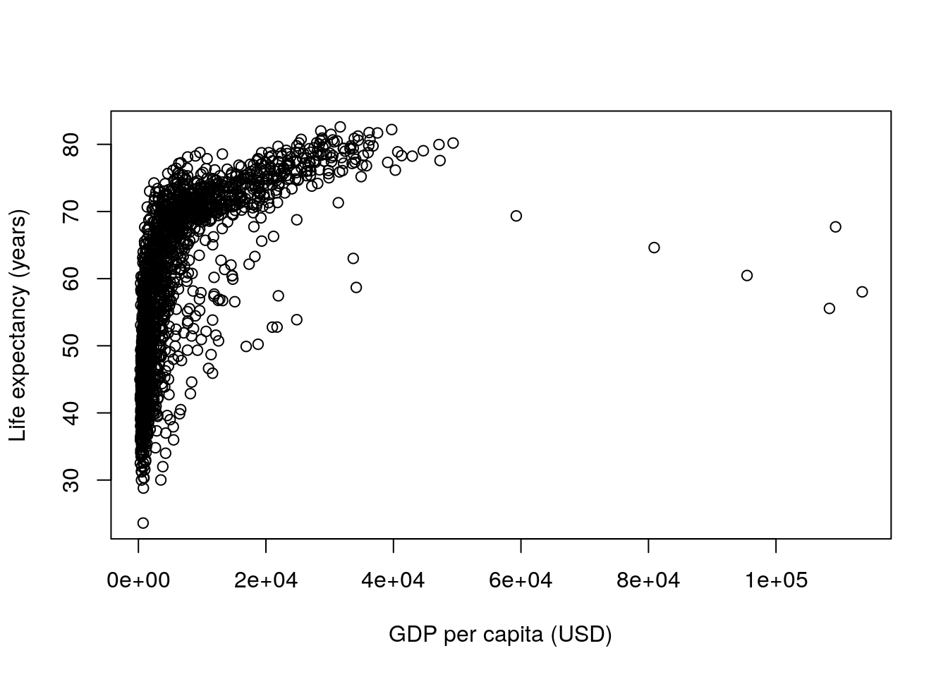

Packages

Packages add functionalities to R and RStudio. There are more than 18,000 available on the official repository: the Comprehensive R Archive Network, or “CRAN”.

You can see the list of installed packages in your “Packages” tab, or by using the library() function without any argument.

We are going to install and load a new package called “praise”. We can do that with the GUI: click the “Install” button in the “Packages” tab (bottom right pane), and search for “praise”.

Notice how it runs an install.packages() command in the console? You can use that too.

If I try running the command praise(), I get an error. That’s because, even though the package is installed, I need to load it every time I start a new R session. The library() function can do that.

library(praise) # load the package
praise() # use a function from the package

## [1] "You are amazing!"

Even though you might need the motivation provided by this function, other packages are more useful for your work.

Let’s take the dplyr package: it is a package that contains a number of function to transform data frames.

Let’s first install dplyr on our computer. In the console, execute the following command:

install.packages("dplyr")

This will take more time than for the praise package, as it is a bigger package that also depends on many other packages.

We can then load the package, and use the filter() function to focus on one part our gapminder dataset:

library(dplyr)

## 
## Attaching package: 'dplyr'

## The following objects are masked from 'package:stats':
## 
##     filter, lag

## The following objects are masked from 'package:base':
## 
##     intersect, setdiff, setequal, union

filter(gapminder, country == "Australia")

##      country year      pop continent lifeExp gdpPercap
## 1  Australia 1952  8691212   Oceania  69.120  10039.60
## 2  Australia 1957  9712569   Oceania  70.330  10949.65
## 3  Australia 1962 10794968   Oceania  70.930  12217.23
## 4  Australia 1967 11872264   Oceania  71.100  14526.12
## 5  Australia 1972 13177000   Oceania  71.930  16788.63
## 6  Australia 1977 14074100   Oceania  73.490  18334.20
## 7  Australia 1982 15184200   Oceania  74.740  19477.01
## 8  Australia 1987 16257249   Oceania  76.320  21888.89
## 9  Australia 1992 17481977   Oceania  77.560  23424.77
## 10 Australia 1997 18565243   Oceania  78.830  26997.94
## 11 Australia 2002 19546792   Oceania  80.370  30687.75
## 12 Australia 2007 20434176   Oceania  81.235  34435.37

This command uses a logical operation to only keep the rows of data that have the value "Australia" in the column country.

Closing RStudio

You can close RStudio after making sure that you saved your script.

When you create a project in RStudio, you create an .Rproj file that gathers information about the state of your project. When you close RStudio, you have the option to save your workspace (i.e. the objects in your environment) as an .Rdata file. The .Rdata file is used to reload your workspace when you open your project again. Projects also bring back whatever source file (e.g. script) you had open, and your command history. You will find your command history in the “History” tab (upper right panel): all the commands that we used should be in there.

If you have a script that contains all your work, it is a good idea not to save your workspace: it makes it less likely to run into errors because of accumulating objects. The script will allow you to get back to where you left it, by executing all the clearly laid-out steps.

The console, on the other hand, only shows a brand new R session when you reopen RStudio. Sessions are not persistent, and a clean one is started when you open your project again, which is why you have to load any extra package your work requires again with the library() function.

What next?

Join this afternoon’s R + OpenStreetMap session
We have a compilation of resources for the rest of your R learning (some of it UQ-specific)
And a cheatsheet of main terms and concepts for R

a very scientifically correct calculation↩︎