This workshop was originally presented at State of the Map 2021.
Introduction
As an interactive, open-source, high-level programming language designed for data science, R is a great fit for dealing with OpenStreetMap data and introducing beginners to reproducible scientific computing. In this workshop, you will learn how you can use a variety of R packages that are ideal to:
- acquire relevant OSM data in a vector format
- clean and process the data
- display it in static and interactive visualisations
- share a visualisation with others
- export the data to other programs for further editing
Most data acquisition, cleaning, processing, visualising and exporting can be done writing an R script. For further refinement of an output, other point-and-click programs (like QGIS) might be required, but storing the bulk of the process in a script allows us to easily reapply the same process on an updated dataset, share the process with others so they can learn from it, and provide supporting evidence when publishing results.
Basic knowledge of R is preferred to follow along this workshop.
If you want to run the commands on your own computer and learn by doing, please make sure you have:
- R installed
- RStudio installed
- the necessary libraries for spatial data processing (see OS-specific instructions)
Outline
In this presentation, we focus on three main packages:
Some important shortcuts for RStudio
- function or dataset help: press F1 with your cursor anywhere in a function name.
- execute from script: Ctrl + Enter
- assignment operator (
<-): Alt + - - pipe (
|>since R 4.1): Ctrl + Shift + M
Acquire data
We want to acquire data about libraries around Meanjin (Brisbane), in Australia. The format we choose is called “simple features”: a convenient spatial format in R, for vector data and associated attributes.
The osmdata package allows us to build Overpass queries to download the data we are interested in. The opq() function (for “overpass query”) can be used to define the bounding box (with Nominatim), and after the pipe operator |>, we can use add_osm_feature() to define the relevant tag.
# load the package
library(osmdata)
# build a query
query <- opq(bbox = "meanjin, australia") |>
  add_osm_feature(key = "amenity", value = "library")
Now that the query is designed, we can send it to Overpass, get the data, and store it as an sf object with osmdata_sf():
libraries <- osmdata_sf(query)Structure of object
We end up with a list of different kinds of vector data, because OSM contains libraries coded as both points and polygons:
In this object, we can see that most libraries in the Meanjin area are stored in OSM as polygons and points. We can do operations on specific parts, for example to see how many libraries there are in each one:
nrow(libraries$osm_points)## [1] 453nrow(libraries$osm_polygons)## [1] 42Now, let’s see the attributes available for libraries coded as points:
names(libraries$osm_points)## [1] "osm_id" "name" "access"
## [4] "addr.city" "addr.country" "addr.full"
## [7] "addr.housenumber" "addr.place" "addr.postcode"
## [10] "addr.state" "addr.street" "addr.suburb"
## [13] "air_conditioning" "alt_name" "amenity"
## [16] "attribution" "contact.email" "contact.phone"
## [19] "contact.website" "description" "entrance"
## [22] "internet_access" "internet_access.fee" "level"
## [25] "note" "opening_hours" "operator"
## [28] "operator.type" "phone" "source"
## [31] "source.date" "source.url" "source_ref"
## [34] "toilets" "toilets.wheelchair" "website"
## [37] "wheelchair" "wheelchair.description" "geometry"You can also explore the dataframe by viewing it:
View(libraries$osm_points)You can find the OSM identifiers in the first column, osm_id. This is what you can use if you want to see the corresponding object on the OSM website. For example, the Indooroopilly Library could be found by putting its ID 262317826 behind the URL https://www.openstreetmap.org/node/.
453 features seems a bit high… Notice that there is a lot of missing data? Many points have no tags, not even amenity=library. Looks like many points are part of polygons, not libraries stored as single points.
Cleaning up
We can remove the points that we are not interested in, with the package dplyr and its function filter():
library(dplyr)
library(sf) # for the filter.sf method
point_libs <- libraries$osm_points |>
  filter(amenity == "library")
39 libraries sounds more realistic!
From polygons to centroids
We have two kinds of vector data: points in point_libs, and polygons in libraries$osm_polygons. We want to process and visualise all libraries in one go, so we should convert everything to points.
The sf package provides many tools to process spatial vector data. One of them is st_centroid(), to get the centre point of a polygon.
library(sf)
centroid_libs <- libraries$osm_polygons |>
  st_centroid()
Note: most function names in the
sfpackage will start withst_, which stands for “space and time”. The plan is to integrate time features in the package.
Now that we have centroids, we can put them in the same object as the other points with dplyr’s bind_rows() function:
all_libs <- bind_rows(centroid_libs, point_libs)bind_rows() is happy to deal with different numbers of columns and will insert NAs as needed. We end up with a total of 57 attribute columns.
You might have to investigate the validity of the data further, for example finding out why some libraries don’t have a name. It could be that the name is simply missing, or that the library tag is duplicated between a point and a polygon.
To only see the ID of the features that don’t have a name:
all_libs |>
  filter(is.na(name)) |>
  pull(osm_id)
## [1] "47415319" "146583077" "330599902" "7416188347"Reproject the data
Currently, the Coordinate Reference System (CRS) in use is EPSG:4326 - WGS 84.
st_crs(all_libs)## Coordinate Reference System:
## User input: EPSG:4326
## wkt:
## GEOGCRS["WGS 84",
## ENSEMBLE["World Geodetic System 1984 ensemble",
## MEMBER["World Geodetic System 1984 (Transit)"],
## MEMBER["World Geodetic System 1984 (G730)"],
## MEMBER["World Geodetic System 1984 (G873)"],
## MEMBER["World Geodetic System 1984 (G1150)"],
## MEMBER["World Geodetic System 1984 (G1674)"],
## MEMBER["World Geodetic System 1984 (G1762)"],
## ELLIPSOID["WGS 84",6378137,298.257223563,
## LENGTHUNIT["metre",1]],
## ENSEMBLEACCURACY[2.0]],
## PRIMEM["Greenwich",0,
## ANGLEUNIT["degree",0.0174532925199433]],
## CS[ellipsoidal,2],
## AXIS["geodetic latitude (Lat)",north,
## ORDER[1],
## ANGLEUNIT["degree",0.0174532925199433]],
## AXIS["geodetic longitude (Lon)",east,
## ORDER[2],
## ANGLEUNIT["degree",0.0174532925199433]],
## USAGE[
## SCOPE["Horizontal component of 3D system."],
## AREA["World."],
## BBOX[-90,-180,90,180]],
## ID["EPSG",4326]]This Geographic Reference System is good for global data, but given that our data is localised, and that we might want to talk about relevant distances, we should reproject the data to a local Projected Reference System (PRS). A good PRS for around Brisbane/Meanjin is “EPSG:7856 - GDA2020 / MGA zone 56”.
# this is a first step that might not be needed,
# but will avoid an error in case of GDAL version mismatch
st_crs(all_libs) <- 4326
all_libs <- st_transform(all_libs, crs = 7856)
If you want to learn more about the static datum GDA2020 (for “Geocentric Datum of Australia 2020”), an upgrade from the previous, less precise GDA94, head to the ICSM website.
Visualise
The default plotting method for an sf object will create facets for the first few columns of attributes.
plot(all_libs)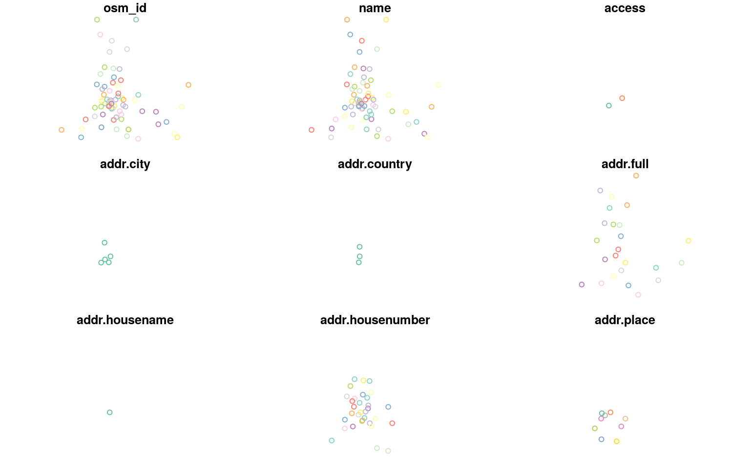
If you just want to have a quick look at the spread of the features on a single plot, you can extract the geometry first:
st_geometry(all_libs) |>
  plot()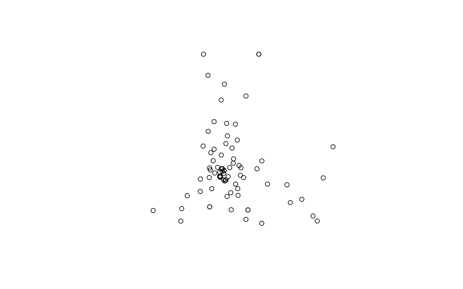
To put the points on a map, a great package is tmap, which can create interactive maps:
library(tmap)
tmap_mode("view")
tm_shape(all_libs) +
  tm_sf()
tm_sf() is useful to quickly visualise an sf object, which can actually contain a combination of points, lines and polygons.
It might be a good idea to show the area of study by also showing the bounding polygon that was used to get the data.
# get a bounding box (we have to extract the multipolygon)
meanjin <- getbb("meanjin, australia", format_out = "sf_polygon")$multipolygon
# also fix the CRS, if needed
st_crs(meanjin) <- 4326
meanjin <- st_transform(meanjin, crs = 7856)
# layer the polygon below the points
tm_shape(meanjin) +
  tm_borders() + # easy way to draw a polygon without a fill
tm_shape(all_libs) +
  tm_dots() # just for point geometries
Notice how the OSM data that was return by Overpass was for the rectangular region that contains the urban area. If we really wanted to focus on only the points contained in the area, we could do a spatial subset:
clipped_libs <- st_intersection(all_libs,
                                st_transform(meanjin, 7856)) # they need the same CRS
Note: there is also a
trim_osmdata()function inosmdatathat does a similar thing.
Only 56 libraries remain.
tm_shape(meanjin) +
  tm_borders() +
tm_shape(clipped_libs) +
  tm_dots()
What if you also want to draw a buffer around your points? We can use st_buffer() to draw a 2-km buffer around each library, and then dissolve them all by using dplyr’s summarise(). You’ll see that many dplyr verbs work very intuitively with sf objects!
library(units)
buffer <- clipped_libs |>
  st_buffer(dist = set_units(2, km)) |>
  summarise()
plot(buffer)
plot(clipped_libs, add = TRUE)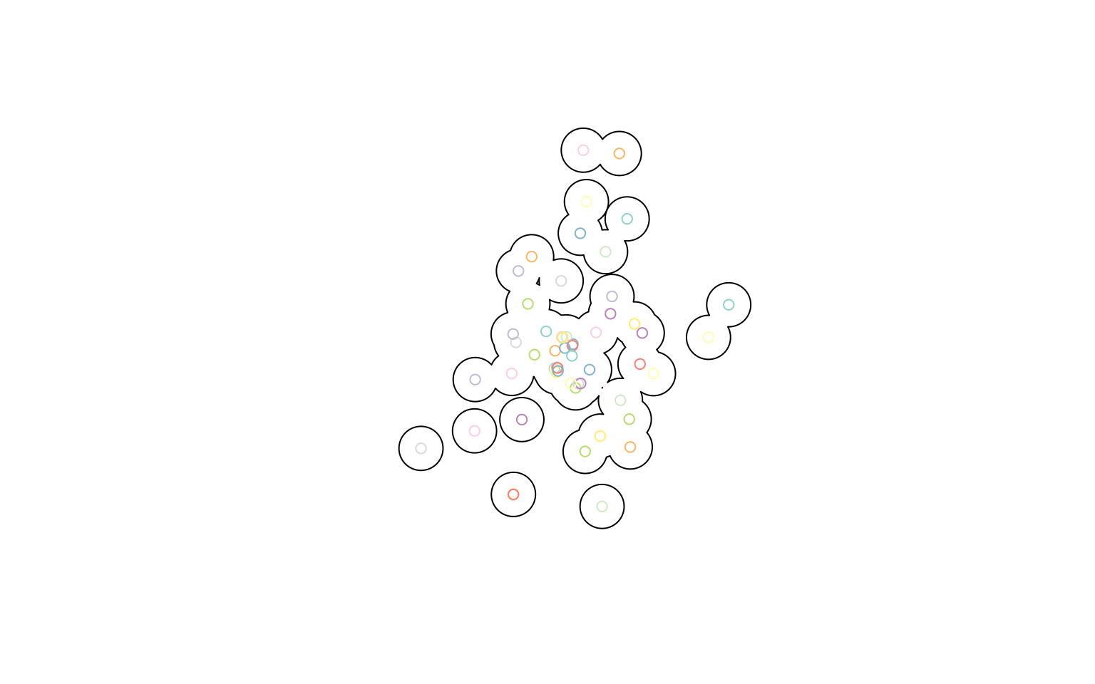
Let’s add our buffers to the interactive map:
tm_shape(meanjin) +
  tm_borders() +
tm_shape(buffer) +
  tm_polygons(col = "pink", alpha = 0.3) +
tm_shape(clipped_libs) +
  tm_dots()
The order of the functions does matters, as they define the order the layers are drawn in.
The default ESRI basemap doesn’t use OSM data, and doesn’t have a precise enough zoom level. You can find a provider name by looking at the providers object, which offers rlength(providers)` options, or explore them visually with the leaflet-extra website.
providers |> names() |> head(20) # just show the first few## [1] "OpenStreetMap" "OpenStreetMap.Mapnik"
## [3] "OpenStreetMap.DE" "OpenStreetMap.CH"
## [5] "OpenStreetMap.France" "OpenStreetMap.HOT"
## [7] "OpenStreetMap.BZH" "OpenSeaMap"
## [9] "OpenPtMap" "OpenTopoMap"
## [11] "OpenRailwayMap" "OpenFireMap"
## [13] "SafeCast" "Thunderforest"
## [15] "Thunderforest.OpenCycleMap" "Thunderforest.Transport"
## [17] "Thunderforest.TransportDark" "Thunderforest.SpinalMap"
## [19] "Thunderforest.Landscape" "Thunderforest.Outdoors"Let’s now refine this visualisation with a few more arguments and functions:
lib_map <- tm_basemap(server = "CartoDB.PositronNoLabels") +
tm_shape(meanjin) +
  tm_borders() +
tm_shape(buffer) +
  tm_polygons(col = "pink", alpha = 0.3) +
tm_shape(clipped_libs) +
  tm_dots(size = 0.1,                       # bigger dots
          col = "toilets",                  # colour by key value
          id = "name",                      # change default tooltip value
          # which variables are in the popup
          popup.vars = c("internet_access", "wheelchair", "operator")) +
  tm_scale_bar() +                          # add a scale bar
  tm_layout(title = "Libraries in Meanjin") # add title
lib_map
Static visualisation
The tmap package allows us to switch between “plot” (the default) and “view” modes.
By switching to “plot” mode again, we can use the same code to create a static plot:
tmap_mode("plot")## tmap mode set to plottinglib_map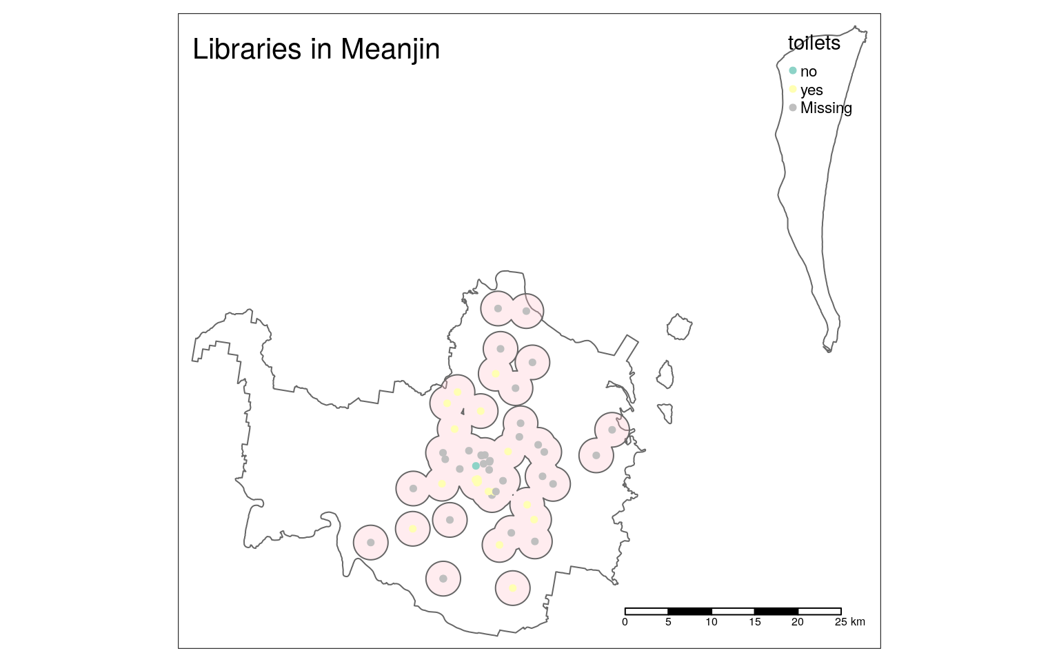
Notice that not all settings can be translated between the different modes. For example, there is no background, the legend does not have an automatic frame, and the scale bar looks different.
For a basemap, we can download a raster image for the right area. For that to work, we need to use the function read_osm() from the package tmaptools (and have the package OpenStreetMap installed as well).
library(tmaptools)
# need the package OpenStreetMap for this to work
bg <- read_osm(meanjin, type = "stamen-watercolor")
You can find the different values for the
typeargument in the documentation:?OpenStreetMap::openmap
We can now use that image using the tm_rgb() function instead of tm_basemap(), and custumise other parts of the plot to make it more readable. In particular, point colours need to contrast with polygon and background colours.
lib_map_static <- tm_shape(bg) +
  tm_rgb(alpha = 0.5) +
tm_shape(meanjin) +
  tm_borders() +
tm_shape(buffer) +
  tm_polygons(col = "grey", alpha = 0.5) +  # a fill that works better
tm_shape(clipped_libs) +
  tm_dots(size = 0.1,
          col = "toilets",
          palette = "Dark2",                # palette that contrasts
          colorNA = "black",                # colour that contrasts
          id = "name",
          popup.vars = c("internet_access", "wheelchair", "operator")) +
  tm_scale_bar() +
  tm_layout(title = "Libraries in Meanjin",
            legend.bg.color = "grey",        # same as buffer
            legend.bg.alpha = 0.5) +         # same as buffer
  tm_credits("© OpenStreetMap contributors") # credits
lib_map_static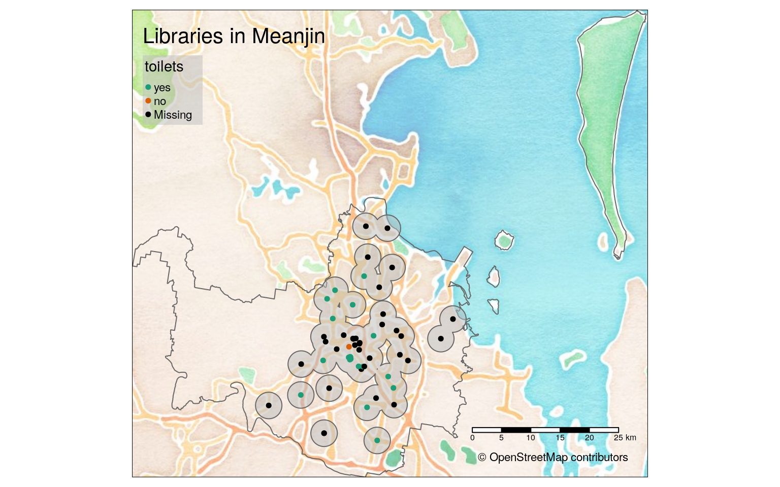
Export a visualisation
The HTML visualisation can be easily exported using the Viewer tab’s Export menu, and the static one using the Plot tab’s Export menu.
However, you can also use a function to automate that:
tmap_save(lib_map, "meanjin_libs.html")
tmap_save(lib_map_static, "meanjin_libs.png")
Export data
To use the data in a different program, you can export in a variety of formats with the function st_write() from the sf package. For example, to export as GeoJSON:
st_write(clipped_libs, "meanjin_libraries.geojson")More advanced queries
If I wanted to have a more thorough look at a variety of places where books can be acquired, I could have built a more complex query:
# public bookcases
public_bookcases <- opq(bbox = "meanjin, australia") |>
  add_osm_feature(key = "amenity", value = "public_bookcase") |>
  osmdata_sf()
# book shops
book_shops <- opq(bbox = "meanjin, australia") |>
  add_osm_feature(key = "shop", value = "books") |>
  osmdata_sf()
# merge the three
where_to_read <- c(libraries, public_bookcases, book_shops)
The reason you couldn’t simply string the different add_osm_feature() calls is that they would be joined with AND: the query would return only features that have all three tags.
For example, if you were only interested in libraries that have toilets, you could use this simpler query:
libs_with_toilets <- opq(bbox = "meanjin, australia") |>
  add_osm_feature(key = "amenity", value = "public_bookcase") |>
  add_osm_feature(key = "toilets", value = "yes") |>
  osmdata_sf()
Other useful packages
osmextractto extract OSM data from downloads sourced from a variety of providers (like Geofabrik, Bbbike or OpenSteetMap.fr).mapsf(successor tocartography), for thematic maps usingsfobjects.
What next?
- Lovelace et al.’s book Geocomputation with R is a wonderful resource for learning more about dealing with spatial data in R
- We have a compilation of resources for the rest of your R learning (some of it UQ-specific)
- And a cheatsheet of main terms and concepts for R
Legal
This workshop, as the name suggests, makes use of OpenStreetMap data, which released under an ODbL licence and is © OpenStreetMap contributors.
This material is released under a CC BY-SA 4.0 licence, which allows you to reuse and remix it, as long as you attribute the source.